지난 시간까지 Propagation of Light라는 제목으로 빛이 매질 속을 진행하며 발생하는 다양한 상호작용 현상에 대해 공부했다. 그렇지만 실제 구체적인 값을 얻을 수는 없었다. 따라서 우리는 electromagnetic approach를 통해, 즉 Maxwell equation과 그 경계조건을 이용해 빛의 상호작용을 조금 더 수식적으로, 구체적으로 이해해보려고 한다.
먼저 다음과 같은 네 가지 (전기장과 자기장 각각 두 가지) 경계조건을 잘 기억해야 한다.
| *Boundary Condition* i) 경계면에 평행한 전기장 혹은 자기장 성분은 경계면에서 연속적이다. ii) 경계면에 수직한 전기장 혹은 자기장 성분은 경계면에서 연속적이다. |
자 이제 다음과 같이 전자기파가 (즉, 빛이) 1번 매질에서 2번 매질로 진행하고 있다고 생각해보자.

전기장은 모니터로부터 나오는 방향으로, 자기장은 표시된 방향으로 나오며 각각 ˆk 방향으로 진행하고 있다고 가정하자. 또 →E 는 boundary surface에 평행하며 tangential한 방향의 성분만 갖는다. →H는 두 성분을 모두 갖는다. 그림과 같은 Free space(i.e., ρf=0,Jf=0)에서, boundary condition과 Maxwell equation을 같이 쓰면 다음과 같다.
{∇⋅→E=0 , ˆn⋅(ε2→E2−ε1→E1)=0∇×→E=−∂→B∂t , ˆn×(→E2−→E1)=0∇⋅→B=0 , ˆn⋅(→B2−→B1)=0∇×→B=με∂→E∂t , ˆn×(1μ2→B2−1μ1→B1)=0
Boundary condition를 정리하면,
{∇⋅→E=0 , ε2→E2n−ε1→E1n=0∇×→E=−∂→B∂t , →E2t−→E1t=0∇⋅→B=0 , →B2n−→B1n=0∇×→B=με∂→E∂t , 1μ2→B2t−1μ1→B1t=0
이제 경계조건을 한 개씩 살펴보자.
1. 처음에 언급한 것 처럼 →E는 tangential한 성분만 갖기 때문에, →E1n=→E2n=0 이다.
2. 두 번째 경계조건에서, →E1t=→E2t 이므로
[→Ei+→Er]t=[→Et]t→Ei+Er=Et
3. 세 번째 경계조건에서, B1n=B2n
4. 마지막 경계조건에서, 1μ1→B1t=1μ2→B2t 이다.
이 때 자기장의 tangential 한 성분은 각각 Hit=−Hicosθi ,Hrt=Hrcosθr, Htt=−Htcosθt 이다. 따라서
1μ1(−Bisinθi+Brsinθr)=1μ2(−Btcosθt)
한편 →E=E0ei(kz−ωt),→B=B0ei(kz−ωt)라고 하면
∇×→E=−ik(−Eyˆx+Exˆy)=−∂→B∂t=iω→B∴
따라서 \left | \vec B \right | = \frac{1}{v} \left | \vec E \right | 이므로 B_t = \frac{1}{v} E = \sqrt{\mu \epsilon} E 이다. 이를 대입하면
\frac{1}{\mu_1} [-\sqrt{\mu_1 \epsilon_1} E_i cos\theta_i + \sqrt{\mu_1 \epsilon_1} E_r cos\theta_r ] = \frac{1}{mu_2} [-\sqrt{\mu_2 \epsilon_2} E_t cos\theta_t] \\ - \sqrt{\frac{\epsilon_1}{\mu_1}} E_i cos\theta_i + \sqrt{\frac{\epsilon_1}{\mu_1}} E_r cos\theta_r = - \sqrt{\frac{\epsilon_2}{\mu_2}} E_t cos\theta_t
여기까지 유도할 수 있다. 여기에 반사법칙 (\theta_i = \theta_r)과 굴절법칙(n_1 sin\theta_i = n_2 sin \theta_t)을 이용해서 두번째와 네번재 경계조건에서 얻은 식을 정리해보면 다음과 같다.
1. \quad E_i + E_r = E_t \to 1+ (\frac{E_r}{E_i}) = \frac{E_t}{E_i}
2. \quad \sqrt{\frac{\epsilon_1}{\mu_1}} E_i cos\theta_i - \sqrt{\frac{\epsilon_1}{\mu_1}}E_r cos\theta_r = \sqrt{\frac{\epsilon_2}{\mu_2}} E_t cos\theta_t \\ \to \ \sqrt{\frac{\epsilon_1}{\mu_1}}cos\theta_i - \sqrt{\frac{\epsilon_1}{\mu_1}}cos\theta_i {\frac{E_r}{E_i}} = \sqrt{\frac{\epsilon_2}{\mu_1}} cos\theta_t (\frac{E_t}{E_i})
이제 위 식을 정리해서 우리는 (\frac{E_r}{E_i})_{\perp} , (\frac{E_t}{E_i})_{\perp} 를 구하려고 한다. 이 두 변수는 각각 반사계수와 투과계수 (혹은 굴절계수) 이다. \frac{E_r}{E_i} \equiv x로 \frac{E_t}{E_i} \equiv y 로 정의하고 위에서 얻은 두 식을 정리하면
1. \quad 1+x =y \\ 2. \quad \sqrt{\frac{\epsilon_1}{\mu_1}}cos\theta_i - \sqrt{\frac{\epsilon_1}{\mu_1}}cos\theta_i x = \sqrt{\frac{\epsilon_2}{\mu_2}} cos\theta_t y
\rightarrow \quad x = (\frac{E_r}{E_i})_{\perp} = \frac{\sqrt{\frac{\epsilon_1}{\mu_1}}cos\theta_i - \sqrt{\frac{\epsilon_2}{\mu_2}}cos\theta_t}{cos\theta_t \sqrt{\frac{\epsilon_1}{\mu_1}}cos\theta_i + \sqrt{\frac{\epsilon_2}{\mu_2}} cos\theta_t} \\ \quad y = (\frac{E_t}{E_i})_{\perp} \frac{2\sqrt{\frac{\epsilon_1}{\mu_1}}cos\theta_i}{\sqrt{\frac{\epsilon_1}{\mu_1}}cos\theta_i+\sqrt{\frac{\epsilon_2}{\mu_2}}cos\theta_t}
이제 거의 다 왔다. 분자 분모에 \mu_1 \mu_2를 곱해주고 \cos \theta_t = \sqrt{1-(\frac{n_1}{n_2})^2 (sin\theta_i) ^2}를 대입하면,
(\frac{E_r}{E_i})_{\perp} = \frac{\mu_2 n_1 cos \theta_i - \mu_1 n_2 \sqrt{1-(\frac{n_1}{n_2})^2 sin\theta_i ^2}}{\mu_2 n_1 cos\theta_i + \mu_1 n_2 \sqrt{1-(\frac{n_1}{n_2})^2 sin\theta_i ^2}} \\ (\frac{E_t}{E_i})_\perp = \frac{2 \mu_2 n_1 cos\theta_i}{\mu_2 n_1 cos\theta_i + \mu_1 n_2 \sqrt{1-(\frac{n_1}{n_2})^2 sin \theta_i ^2}}
Fresnel equations 중 두 가지를 구했다.
위에서 구한것과 비슷한 방식으로 \vec H 가 모니터에서 나오고, \vec E가 \hat{n}, \hat{t} 방향을 모두 갖는 경우도 생각해 볼 수 있다. 이 경우도 마찬가지로 Maxwell equation과 boundary condition을 이용해 유도할 수 있다.
(작성중)
--
다음 게시글에서는 Fresnel Equations의 의미를 알아본다.